Uniform density runs, sorted on initial position

I went back to the original 4 cases where I varied the initial conditions.  The initial density profile is uniform, and the particles lie exactly on a grid.  Each run has 10k particles, and I have repeated it 4 times to get error bars on the final density profile.  Here is a plot to remind you of what the different initial conditions were:

Runs 1 and 3 behaved very similarly in their evolution, forming a single object that winds up and collapses into the final virialized object.  Runs 2 (with the inflection point in the initial velocities) and 4 (which was initially expanding rather than contracting) were similar to one another in that they each formed 2 distinct objects that later merged to form the final product.  What you will see in this post is that the fate of the innermost and outermost particles depends greatly on the formation history, although the final density profile of the remnant does not. 

Here are the final phase space configurations (transformed so you can see the interior parts too) of the 4 runs.  Reddish brown particles started farthest out, and blue and green particles began life farthest in:

Here we see that for initial conditions 2 and 4, the ones in which there was a merger event, the innermost particles are driven to the far exterior of the object, and the innermost particles of the remnant started life in the outermost ring.   In contrast, for the monolithic cases, the innermost particles of the remnant come from a mixture of intermediate and inner rings, and just as we saw in the power law cases, the distribution of the inner particles is not isotropic in phase space.

Here are plots the initial vs. final positions and velocities of the particles:

These show that there is a very specific band of the initial particles that wind up in the middle of the remnant, in the merger cases.  Also, the "tail" that we were seeing int he velocity plots of the power law cases does not seem to appear here.

Finally, just to complete the story, here are plots of the final density profile of the 4 different runs.

 

Here it is evident that the monolithic cases scale as $r^{-1/2}$ over more decades than the cases with merger events, but even the cases where the inner particles come mostly from the outer layers scale quite convincingly (at least by eye) like $r^{-1/2}$.

IP sorting for all the power law runs

Got a little time during nap today to make more plots.  Here are plots comparing the fate of particles in different initial positions for four different runs:  $\rho \propto x^{-1/2}$ (you saw these plots yesterday), $\rho \propto x^{-0.8}$, $\rho \propto x^{-0.3}$  and $\rho \propto x^{+0.5}$.  I made the log and polar versions of the plots, but not the zoom ins.  Here they are, labels are at the top.

 

 

 

General trends:

1)  The steeper the initial power law slope, the farther out the origin of the innermost particles at the final configuration.
2)  The steeper the initial power law slope, the more asymmetric the final configuration is in phase space.
3)  If the density of the initial object increases with radius rather than decreasing, it is the outermost particles that wind up in the middle, and the innermost wind up around the ouside in phase space.
4)  For runs with a negative power law slope, although they maintain their density scaling in the intermediate range, it seems like almost none of the particles collapse in farther than the position of the innermost particle at the beginning of the run (only in the very shallow case do particles make it farther in).

Sorting by inital positions

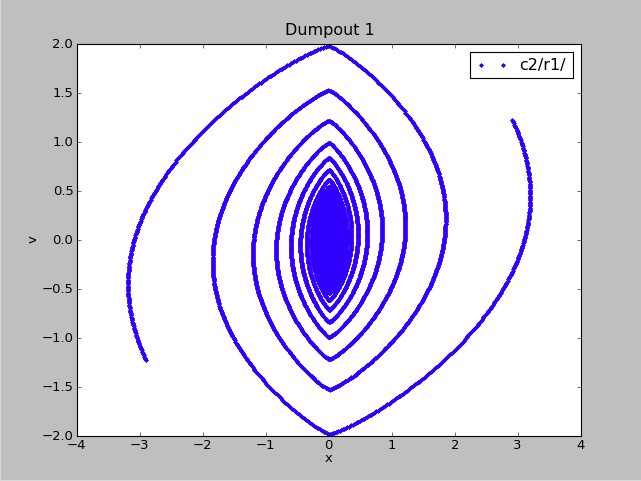
I have added a feature to Walter's code, namely each particle carries about a memory of where it started it's life.   I have done several runs, but all of the following plots refer to initial conditions that were a power law density profile with $\rho \propto x^{-1/2}$.   I have defined 5 logarithmic bins in the particle initial positions.  Below is the phase space diagram, with different colors representing particles that started in different initial positions, the reddish brown ones began life the bin farthest out, and the dark blue began life in the innermost bin.  Each plot is zoomed in from it's predecessor (you can click on the plots to view them larger):

Just for illustration, here are the same types of plots, but for the initial conditions (note the aspect ratio is no longer square):

To get a better idea of how the different colors are distributed around phase space, I did a transformation on these data to fit all the information onto a single plot.  Below I have defined a distance in phase space which is $r=\sqrt{x^2 + v^2}$.  Then instead of plotting $(r,\theta)$, I plot $(r^{0.1}, \theta)$ so that we can see the inner parts. 

Here are the initial conditions in this view:

These plots demonstrate that the outermost bins retain their identity, but the inner bins get mixed in the ordering of their positions.  All of the velocities increase, but the inner bins tend to have only high velocities and small positions.  The phase space orbits for the outer particles and inner particles seem qualitatively different.  This result is robust to the phase of the winding:  I checked that it holds true for the last several time dumps, and also for different runs of the same initial conditions (different runs have different numbers of particles).

Another useful view is to look at scatter plots of $|x_i|$ versus $|x_f|$ and $|v_i|$ versus $|v_f|$.  Here they are, the black lines show $x_f=x_i$ and the analogous for the velocity.

You can see that the positions on average are collapsing inward, as expected, but the innermost particles do not collapse inward as much as some of their outer counterparts, in fact the very innermost ones seem to be thrown out of the central region.  The velocities are all increasing, with the innermost particles seeing the largest increase in velocity.  This basic structure is set up very early in the run, here is the first time dump after the start of the run, at 20 ATUs.

I was puzzled about that tail in the outer particles, I thought maybe looking at these plots in a slightly different way might shed some light.  Here are $x_i$ versus $x_f$ and $v_i$ versus $v_f$ plots, where again I just zoom in rather than doing the polar trick.  The axes have the same ranges as in the beginning of this post (except v_initial, which I scale down in the same proportions):

So you can see the velocity tail in a different form, in the first of these, I am still thinking aobut why it's there.  The innermost bins are doing something qualitatively different than the outer three, in my opinion.

There are still many more plots to make, I will start checking some of the other power laws.  Also, if I want to do warm runs, I need to repeat the modification to Walter's code, adding one more field (and since it's the last available bit, that is it, can't add any more data to carry around without doing something hard).    I will try and make some more plots this weekend, have good one.

Cold runs, recentered

Here are the power law cold runs, done with the updated recentering algorithm.   The initial conditions for these runs is $\rho \propto x^a$ with $a=-0.5, -0.7, -0.8, -0.3, +0.5$  They all have 10k particles.

Also, here is the run with $a=-0.2$, and 80k particles.

The cold runs with slope <-0.5 appear to exhibit the same flattening in the center as the warm runs.  Qualitatively, the warm and cold appear indistinguishable.  However, runs with initial slope >-0.5 do not appear to retain their original scaling, and they do not go to the attractor behavior, even when they are cold.   The run with initial slope >0 appears to do something like the attractor behavior, oddly enough. 

Recentering fixed

I have modified my code that generates the density plots.  Whereas before, the scheme was

1) Bin up so that there are N particles per bin
2) Compute the density
3) Find the position of the density maximum
4) shift all the particle positions so that the density maximum is at x=0
5) Bin up again with N particles per bin
6) Compute the density and plot

This worked relatively well for the runs where the particles began in an equally spaced configuration, but once I started the initial conditions with a power law, suddenly a much higher fraction of the particles wind up in the middle, but the offset from 0 was a similar magnitude as the equally spaced case.  Therefore, for the power law runs, when I got to step 5, sometimes with the new binning, the density maximum was again off-shifted from zero by some number of bins.  I have solved this issue by iterating the process until the shift is at most only one bin, then I stop.   Here are the plots for the warm runs, I think they are significantly improved, and I am also relieved to see the appearance of the flattening in the center of the -0.8 run.  I am somewhat surprised that it did not show up in the center of the -0.5 run.

I think it is advisable to remake several of the key plots using the new algorithm, even for the runs that were of constant initial density.  I will do so, and post them in the next post.

Code doing strange things.

I was investigating the part of my analysis that is responsible for recentering on the middle of the collapsed object.  I have not figured out whether it is working the way I expect it to, or not, but in the process I discovered that the code is behaving strangely in some of the runs.  For example, here is a normal sequence, in the warm sim with initial density profile $x^{-0.8}$, dumping out the particles every 20 ATUs (time units).  This run had 10004 particles in it.

Now here is a run that crashed (in the sense that all the positions were NAN, not in the hanging up on timestep 0, which is the other failure mode).  The only difference between this run and the previous one is that this one had 10007 particles, rather than 10004.  And of course the thermal part of the velocity has a random component.  What happens is very hard to explain:

Note the x axis.  The very next time dump was all NAN.  10010, 10013, 10016, and 10019 particles all looked identical to the blue run above, and ran in a well behaved way until the end.    If you zoom into one of those regions in Dumpout 3 of the crashing run, it looks like this:

So some of the coherence in the structure is still being maintained...   Thoughts anyone?